Lecture 10 - Statistical Data Analysis

• 10.1 Descriptive Statistics

  • 10.1.1 Measures of Central Tendency

  • 10.1.2 Measures of Variability

  • 10.1.3 Summary of Descriptive Statistics

  • 10.1.4 Measures of Correlation

• 10.2 Inferential Statistics

  • 10.2.1 Linear Regression

  • 10.2.2 Standard Error of the Mean

  • 10.2.3 Confidence Intervals

  • 10.2.4 Hypothesis Testing

• References

Statistical data analysis is an essential aspect of data science and machine learning. Via statistical data analysis, we can obtain meaningful insights from datasets, make predictions, and inform decision-making. In this lecture, we will cover Python libraries for statistical analysis, including the calculation of descriptive statistics and inferential statistics. Descriptive statistics involves methods for summarizing and organizing data to describe their main features and characteristics. The data summarization is typically in the form of summary statistics and visualization techniques. Inferential statistics involves methods for making inferences or predictions about a population based on a sample of data.

10.1 Descriptive Statistics

Descriptive statistics provide basic summaries about a dataset and insights into the characteristics of a dataset. In Data Science, descriptive statistics are often the first step in data exploration, enabling to understand the underlying patterns of the data, detect anomalies, and form hypotheses for further analysis. The initial examination is important for guiding subsequent analyses, which may involve inferential statistics or machine learning model development.

Providing data summaries via descriptive statistics can involve: * Calculating quantitative measures that describe and summarize the data numerically. * Using visualization techniques to present data distributions and relationships with charts and plots.

We can apply descriptive statistics to analyze a single variable (feature), or the relationship between multiple variables (features) within a dataset. The type of analysis that focuses on understanding the basic characteristics of a single feature in isolation is referred to as uinivariate analysis. Statistical analysis that examines the relationships and patterns among multiple variables is multivariate analysis. The special case of examining the statistical relationships among a pair of variables is called bivariate analysis.

Quantitative descriptive statistics measures are typically categorized into:

• Measures of central tendency, such as the mean, mode, and median, describe the center of the data and indicate where most data points are concentrated.

• Measures of variability, such as the range, variance, and standard deviation, quantify the spread or dispersion of the data and show how much the data points differ from the central values.

• Measures of correlation, such as correlation coefficient and covariance, quantify the relationships between variables in a dataset.

Additionally, measures like skewness and kurtosis describe the shape of the data distribution, highlighting asymmetry or the presence of outliers in the data.

10.1.1 Measures of Central Tendency

The measures of central tendency describe the central or middle values of a dataset, i.e., the location where most data points are concentrated.

The measures of central tendency include:

• Mean

• Median

• Mode

• Weighted mean

• Geometric mean

• Harmonic mean

Mean

The mean of a sample drawn from a population is the arithmetic average of all elements in a dataset. It is also called the sample arithmetic mean or simply the average.

The mean of a dataset 𝑥 is mathematically expressed as:

\(\overline{x} = \frac{\sum_{i=1}^{n} x_i}{n}\)

In Python we can calculate the mean of a sequence of items using the built-in functions sum() and len().

x = [8.0, 1, 2.5, 4, 28.0]

mean = sum(x) / len(x)
mean

8.7

Alternatively, it may be more convenient to import the built-in Python library statistics for calculating descriptive statistics and for performing other types of statistical analyses.

import statistics

mean = statistics.mean(x)
mean

8.7

As we learned in the previous lectures, the libraries NumPy and pandas allow calculating descriptive statistics for data in the form of ndarrays and DataFrames.

import numpy as np

# NumPy
y = np.array(x)

mean = np.mean(y)
mean

8.7

The average() function in NumPy can also be used to calculate the mean of an array.

# NumPy
mean = np.average(y)
mean

8.7

import pandas as pd

# pandas
z = pd.Series(x)

mean = z.mean()
mean

8.7

A limitation of the mean is its sensitivity to outliers in the dataset having extremely high or low values. Also, it may not accurately reflect the central tendency if the dataset is skewed.

Median

The median of a sample is the middle element of the sorted elements. The dataset can be sorted in increasing or decreasing order. If the number of elements \(𝑛\) of the dataset is odd, the median is the value at the middle position. If \(𝑛\) is even, the median is the arithmetic mean of the two values in the middle. For example, for the data points (2, 4, 1, 8, 9), the sorted dataset is (1, 2, 4, 8, 9), and the median value is 4. If the data points are (2, 4, 1, 8), the sorted dataset is (1, 2, 4, 8), and the median is 3, obtained as the average of the two middle elements 2 and 4.

To calculate the median in native Python, we can write a simple function based on the above description. However, to avoid any errors in our code, we can simply use the implemented function from the statistics library. The sorted version of the above list x is (1, 2.5, 4, 8.0, 28.0), therefore, the median is the element in the middle, which is 4.

# statistics module
median = statistics.median(x)
median

4

Numpy and pandas also provide a median function for this purpose.

# NumPy
median = np.median(y)
print('NumPy:', median)

# pandas
median = z.median()
print('pandas:', median)

NumPy: 4.0
pandas: 4.0

The median is less sensitive to outliers compared to the mean, and therefore, it is considered a more robust measure of central tendency. The median is also particularly useful for skewed distributions.

Mode

The mode of a sample is the value in the dataset that occurs most frequently. For example, in the set that contains the points (2, 3, 2, 8, 12), the number 2 is the mode because it occurs twice. In general, a dataset can have multiple values that occur the most frequently, in which case it is referred to as a multimodal dataset (e.g., if a dataset has two modes, it is called bimodal).

 u = [2, 3, 2, 8, 12]

# statistics
mode = statistics.mode(u)
print('statistics:', mode)

statistics: 2

Note that NumPy does not have a built-in mode function. For this purpose, we can use the scipy.stats module in the SciPy library for scientific calculations which is implemented on top of NumPy. The output includes the value of the mode, and the number of counts it occurs in the dataset.

# NumPy
import scipy
mode = scipy.stats.mode(u)
print('NumPy:', mode)

NumPy: ModeResult(mode=2, count=2)

We can use pandas to calculate the mode as well. Pandas returns a series with all modes in the dataset, and in this case, the only mode is 2, and it has index 0.

# pandas
w = pd.Series(u)
mode = w.mode()
print('pandas:', mode)

pandas: 0    2
dtype: int64

Let’s see another example of a sequence with two modes. Note that the mode() function in the statistics library returns only a single mode, and the multimode() function returns more than one modal value, as shown in the next cell. Therefore, it is preferred to use the multimode() function to avoid missing multimodality in the data.

v = [12, 15, 12, 15, 21, 15, 12]

# statistics
mode = statistics.mode(v)
print('statistics:', mode)

statistics: 12

# statistics
mode = statistics.multimode(v)
print('statistics:', mode)

statistics: [12, 15]

The next cell shows the same example with NumPy and pandas. Note that NumPy returned only one mode, and it does not have a function for dealing with multiple modes. On the other hand, pandas returned both modes.

# NumPy
mode = scipy.stats.mode(v)
print('NumPy:', mode)

# pandas
w = pd.Series(v)
mode = w.mode()
print('\npandas:', mode)

NumPy: ModeResult(mode=12, count=3)

pandas: 0    12
1    15
dtype: int64

Weighted Mean

The weighted mean is a generalization of the arithmetic mean that enables to assign a weight to each data point that quantifies the relative contribution of the data point to the result. It is also called weighted arithmetic mean or weighted average.

If we denote the weight \(𝑤_i\) that is assigned to data point \(𝑥_i\) of the dataset, the weighted mean is obtained by multiplying each data point with the corresponding weight, summing all the products, and dividing the sum with the sum of the weights:

\(\overline{x}_\text{weighted} = \frac{\sum_{i=1}^{n} w_i x_i}{\sum_{i=1}^{n} w_i}\)

The weighted mean is very useful when we need to calculate the mean of a dataset containing items that occur with given relative frequencies. In this case, we consider the frequencies as the weights of the individual data points.

The libraries statistics and pandas do not have functions for calculating the weighted mean. However, it can be easily applied in Python as the example in the next cell.

x = [8.0, 1, 2.5, 4, 28.0]
w = [0.1, 0.2, 0.3, 0.25, 0.15]

# Python
wmean = sum(w[i] * x[i] for i in range(len(x))) / sum(w)
wmean

6.95

In NumPy, the average function allows to assign weights and calculate the weighted mean.

# NumPy
wmean = np.average(z, weights=w)
wmean

6.95

Harmonic Mean

The harmonic mean is the reciprocal of the mean of the reciprocals of all items in the dataset, i.e.:

\(\overline{x}_\text{harmonic} = \frac{𝑛}{\sum_{i=1}^{n}\frac{1}{𝑥_i}}\)

One variant of pure Python implementation of the harmonic mean is as follows.

# Python
hmean = len(x) / sum(1/item for item in x)
hmean

2.7613412228796843

We can also calculate this measure with statistics.harmonic_mean().

# statistics
hmean = statistics.harmonic_mean(x)
hmean

2.7613412228796843

Another way to calculate the harmonic mean is by using scipy.stats.hmean().

# SciPy
scipy.stats.hmean(y)

2.7613412228796843

Geometric Mean

The geometric mean is the 𝑛-th root of the product of all 𝑛 elements \(𝑥_i\) in a dataset:

\(\overline{x}_\text{geometric} = \sqrt[n]{\prod_{i=1}^{n} x_i}\)

It can be calculated by statistics.geometric_mean() and scipy.stats.gmean().

# statistics
gmean = statistics.geometric_mean(x)
gmean

4.67788567485604

# SciPy
scipy.stats.gmean(y)

4.67788567485604

10.1.2 Measures of Variability

The measures of central tendency are not sufficient to describe data, and we also need the measures of variability that quantify the spread of data points.

Measures of variability include:

• Range

• Interquartile range

• Variance

• Standard deviation

• Skewness

Range

The range of a dataset is the difference between the maximum and minimum elements.

To calculate the range, we can use max() and min() from the Python standard library.

In NumPy, we can use np.ptp() (peak-to-peak) to calculate the range directly, or via np.max() and np.min().

Similarly, in pandas we can use .max() and .min().

# Python
range_x = max(x) - min(x)
print('Python:', range_x)

# NumPy
range_y = np.ptp(y)
print('NumPy:', range_y)

# NumPy
range_y = np.max(y) - np.min(y)
print('NumPy:', range_y)

# pandas
range_z = z.max() - z.min()
print('pandas:', range_z)

Python: 27.0
NumPy: 27.0
NumPy: 27.0
pandas: 27.0

When working with range, we need to recall that this statistic is sensitive to outliers in the dataset.

Interquartile Range

The interquartile range (IQR) is the difference between the first and third quartiles. More specifically, IQR is calculated as the difference between the 25th percentile (first quartile) and 75th percentile (third quartile).

A dataset has three quartiles, which divide the dataset into four parts. The first quartile (Q1) is the 25th percentile, and it divides approximately 25% of the smallest items from the rest of the dataset. The second quartile (Q2) is the 50th percentile, or the median. The third quartile (Q3) is the 75th percentile, and it divides approximately 25% of the largest items from the rest of the dataset. In summary, approximately 25% of the items lie between the first and second quartiles, and another 25% lie between the second and third quartiles.

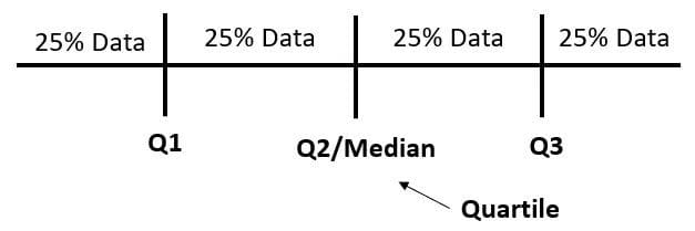Figure: Data by quartiles. Source: [6].

In general, quantiles divide the dataset into equal-sized intervals. An example of quantiles are the quartiles. The type of quantiles that divide the dataset into 100 equal parts are called percentiles. However, quantiles are often referred to as percentiles.

The 10th percentile is the value that is less than or equal to 10% of the data. Consequently, 90% of the elements are greater than or equal to the 10th percentile.

NumPy and pandas provide functions for calculating quantiles. Examples for calculating 10th and 75th quantiles (percentiles) are shown in the next cells.

# NumPy
quantile10th = np.quantile(y, 0.10)
print('NumPy:', quantile10th)

# pandas
quantile10th  = z.quantile(0.10)
print('pandas:', quantile10th)

NumPy: 1.6
pandas: 1.6

# NumPy
quantile75th = np.quantile(y, 0.75)
print('NumPy:', quantile75th)

# pandas
quantile75th  = z.quantile(0.75)
print('pandas:', quantile75th)

NumPy: 8.0
pandas: 8.0

In NumPy there is also a percentile() function which expects the argument to be between 0 and 100, whereas the quantile() function expects the argument to be between 0 and 1.

# NumPy
quantile75th = np.percentile(y, 75)
print('NumPy:', quantile75th)

NumPy: 8.0

To calculate IQR, we can first calculate the first and third quartiles (i.e., 25th and 75th percentiles), and afterward take their difference.

# NumPy
quartiles = np.quantile(y, [0.25, 0.75])
interquartile_range = quartiles[1] - quartiles[0]
print('NumPy:', interquartile_range)

# pandas
quartiles = z.quantile([0.25, 0.75])
interquartile_range = quartiles[0.75] - quartiles[0.25]
print('pandas:', interquartile_range)

NumPy: 5.5
pandas: 5.5

Variance

The sample variance quantifies the spread of the data. It shows numerically how far the data points are from the mean of the dataset. It is calculated as the average of the squared differences from the mean. We can express the sample variance of a dataset with \(𝑛\) elements mathematically as:

\(s^2 = \frac{\sum_{i=1}^{n} (x_i - \overline{x})^2}{n - 1}\)

where \(\overline{x}\) is the sample mean. To denote population variance, the notation \(\sigma^2\) is commonly used.

We can calculate the variance using the function statistics.variance(), in NumPy with np.var(), and in pandas with .var().

# statistics
var = statistics.variance(x)
print('Python:', var)

# NumPy
var = np.var(y, ddof=1)
print('NumPy:', var)

# pandas
var = z.var(ddof=1)
print('pandas:', var)

Python: 123.2
NumPy: 123.19999999999999
pandas: 123.19999999999999

In NumPy and pandas, the parameter ddof=1 sets the delta degrees of freedom to 1. This parameter allows the calculation of \(s^2\) with \(𝑛 − 1\) in the denominator instead of \(𝑛\). By using \(𝑛 − 1\) for the variance of a sample, we account for the bias in estimating the population variance, and compensate for the fact that the sample mean is used as an approximation of the true population mean. This adjustment (called Bessel’s correction) compensates for the fact that the sample is likely to underestimate the true population variance. To calculate the variance of a population, we can set the delta degrees of freedom to 0 in the above codes.

Variance quantifies the spread of the data in squared units, which can make the interpretation less intuitive.

Standard Deviation

The sample standard deviation is the positive square root of the sample variance.

\(s = \sqrt{\frac{\sum_{i=1}^{n} (x_i - \overline{x})^2}{n - 1}}\)

The standard deviation is often more convenient to work with than the variance, because it has the same unit as the data points.

Although we can calculate the standard deviation simply by taking the square root of the variance, almost all libraries have a separate std() or stdev() function for this purpose.

# statistics
std = statistics.stdev(x)
print('Python:', std )

# NumPy
std = np.std(y, ddof=1)
print('NumPy:', std)

# pandas
std = z.std(ddof=1)
print('pandas:', std )

Python: 11.099549540409287
NumPy: 11.099549540409285
pandas: 11.099549540409285

Skewness

The sample skewness measures the asymmetry of a dataset. The figure below illustrates skewness. A dataset is negatively skewed if it tends to have a lot of extremely small values (i.e., the lower tail is longer than the upper tail) and not so many extremely large values (left subfigure). On the other hand, if there are more extremely large values than extremely small ones (right subfigure) we say that the dataset is positively skewed. The formula for the skewness of a dataset is as follows:

\(\text{skew} = \frac{\sum_{i=1}^{n} (x_i - \overline{x})^3}{n s^3}\)

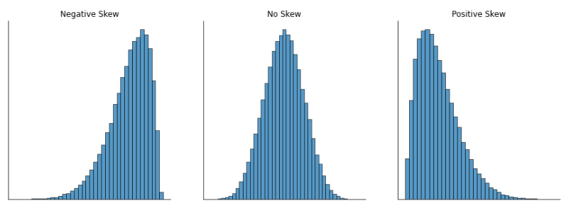Figure: Skewness of a sample. Source: [2].

We can calculate skewness by using the method .skew() in pandas and scipy.stats.skew() can be used with NumPy arrays. The parameter bias=False in the codes indicates to use the unbiased estimation for a sample variance by applying the correction factor (mentioned in the section on variance).

# SciPy
skew = scipy.stats.skew(y, bias=False)
print('SciPy:', skew)

# pandas
skew = z.skew()
print('pandas:', skew)

SciPy: 1.9470432273905927
pandas: 1.9470432273905924

10.1.3 Summary of Descriptive Statistics

The library SciPy allows to list descriptive statistics with the function scipy.stats.describe(), as shown in the next cell. The value nobs refers to the number of observations in the dataset, and the rest of the values are self-explanatory. One statistic that we didn’t explain is kurtosis, which quantifies the “pointness” of a dataset, but it is less frequently used in practice. A dataset that is flat has negative kurtosis, and a dataset that is pointy has positive kurtosis.

# SciPy
scipy.stats.describe(y, ddof=1, bias=False)

DescribeResult(nobs=5, minmax=(1.0, 28.0), mean=8.7, variance=123.19999999999999, skewness=1.9470432273905927, kurtosis=3.878019618875446)

In pandas we can use the method describe() to list descriptive statistics. As we mentioned in the lecture on pandas, for a DataFrame describe() returns descriptive statistics for all columns in the DataFrame that have numerical values.

# pandas
z.describe()

count     5.00000
mean      8.70000
std      11.09955
min       1.00000
25%       2.50000
50%       4.00000
75%       8.00000
max      28.00000
dtype: float64

10.1.4 Measures of Correlation

When performing data analysis, we often need to examine and describe the relationship between the values of two variables (features) in a dataset. If the variables are denoted 𝑥 and 𝑦, we can create pairs of corresponding elements (𝑥₁, 𝑦₁), (𝑥₂, 𝑦₂), and so on, and examine the correlation between the variables.

In general, based on the relationship between the pairs of data points, we can identify the following types of correlation:

• Negative correlation, exists when larger values of 𝑥 correspond to smaller values of 𝑦 and vice versa (left subfigure).

• Weak or no correlation, exists if there is no such apparent relationship (middle subfigure).

• Positive correlation, exists when larger values of 𝑥 correspond to larger values of 𝑦 and vice versa (right subfigure).

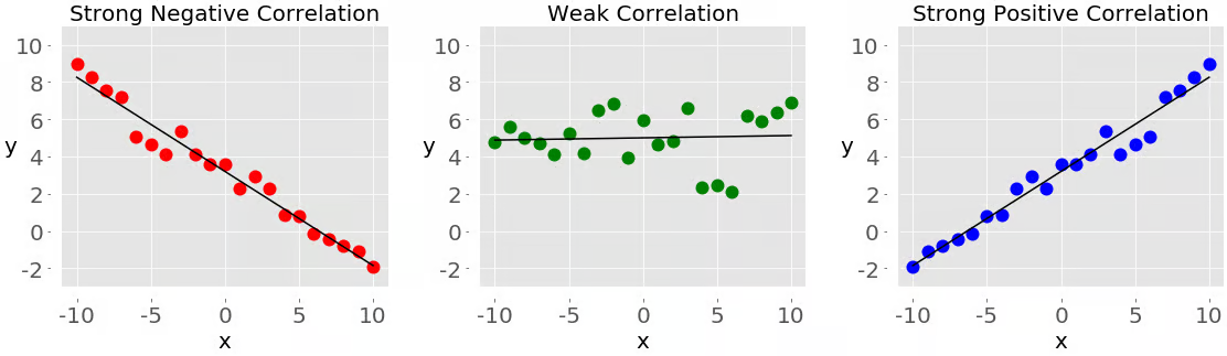Figure: Correlation between two variables. Source: [1].

Two statistics that measure the correlation between datasets are covariance and correlation coefficient.

Covariance

The sample covariance is a measure that quantifies the strength and direction of a relationship between a pair of variables.

• If the correlation is positive, the covariance is positive. A stronger relationship corresponds to a higher value of the covariance.

• If the correlation is negative, the covariance is negative. A stronger relationship corresponds to a lower value of the covariance.

• If the correlation is weak, the covariance is close to zero.

The covariance of variables 𝑥 and 𝑦 is mathematically defined as:

\(s_{xy} = \frac{\sum_{i=1}^{n} (x_i - \overline{x}) (y_i - \overline{y})}{n - 1}\)

Therefore, the covariance of two identical variables is actually the variance, i.e., \(s_{xx} = {\sum_{i} (x_i - \overline{x})^2}/{(n - 1)}=(s_{x})^2\). Or, we can say that the covariance is a generalization of the concept of variance to two or more variables.

To show the calculation of the covariance in Python, let’s create two variables and convert them to NumPy arrays and pandas series.

x = list(range(-10, 11))
y = [0, 2, 2, 2, 2, 3, 3, 6, 7, 4, 7, 6, 6, 9, 4, 5, 5, 10, 11, 12, 14]
xarr, yarr = np.array(x), np.array(y)
xseries, yseries = pd.Series(x), pd.Series(y)

Let’s plot the two lists. We can notice a positive correlation in the plot.

import matplotlib.pyplot as plt

plt.plot(x,y)
plt.xlabel('x')
plt.ylabel('y')
plt.show()

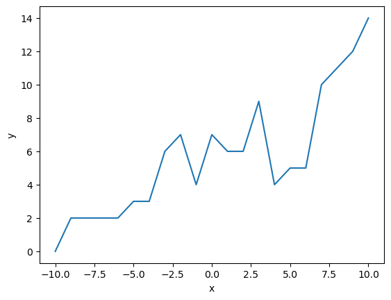
The covariances between variables are often combined into a covariance matrix. For example, to calculate the covariance matrix in NumPy, we can use the function cov().

# NumPy
cov_matrix = np.cov(xarr, yarr)
print('NumPy:', cov_matrix)

NumPy: [[38.5        19.95      ]
 [19.95       13.91428571]]

The elements in the covariance matrix are:

\(\mathrm{covariance\_matrix} = \begin{bmatrix} \text{cov}(x,x) & \text{cov}(x,y) \\ \text{cov}(y,x) & \text{cov}(y,y) \end{bmatrix}\)

Note that the covariance matrix is symmetric, i.e., the off-diagonal elements cov(x,y)\(=s_{xy}\) and cov(y,x)\(=s_{yx}\) are equal.

In this case, the element cov(x,y) = 19.95 suggests a positive correlation between x and y, since the values of y increase with the increase in the values of x.

Note in the cell below that the element cov(x,x) = \(s_{xx}\) is equal to the variance of x (that is \(s_{x}^2\)), and the element cov(y,y)\(=s_{yy}\) is equal to the variance of y (that is \(s_{y}^2\)).

# NumPy
print(xarr.var(ddof=1))
print(yarr.var(ddof=1))

38.5
13.914285714285711

In pandas the method .cov() returns the covariance between two Series objects.

# pandas
cov_xy = xseries.cov(yseries)
cov_xy

19.95

Correlation Coefficient

The correlation coefficient, also known as Pearson correlation coefficient, is another important measure of correlation. It is commonly denoted by the symbol 𝑟, and it is calculated as:

\(r = \frac{s_{xy}}{s_{x}s_{y}}\)

The correlation coefficient is equal to the covariance of the variables \(s_{xy}\) divided by the standard deviations of \(x\) and \(y\). Or, we can say that the correlation coefficient is a measure of standardized covariance. The standardization makes the coefficient in the range from -1 to 1.

Examples of variables with different values of the correlation coefficient are shown in the figure below.

• The value r = −1 is the minimum possible value of 𝑟, and corresponds to a perfect negative linear relationship between variables.

• The value 𝑟 < 0 indicates negative correlation. The more the data is spread, the weaker the correlation is.

• The value r = 0 means that the correlation between the variables is weak.

• The value 𝑟 > 0 indicates positive correlation.

The maximum possible value of 𝑟 is 1, and corresponds to a perfect positive linear relationship between variables.

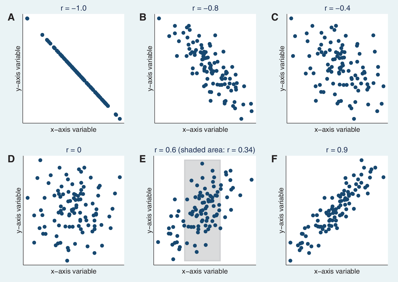Figure: Correlation coefficient \(r\). Source: [3]

To calculate the correlation coefficient, we can use pearsonr() in scipy.stats. It returns both the correlation coefficient and the 𝑝-value. In the next cell, the correlation coefficient is 0.86, indicating strong correlation between the variables x and y. A small 𝑝-value indicates that there is statistically significant evidence that there is a linear correlation between the variables.

# SciPy
scipy.stats.pearsonr(xarr, yarr)

PearsonRResult(statistic=0.861950005631606, pvalue=5.122760847201132e-07)

Similar to the covariance matrix, in NumPy the function np.corrcoef() returns the correlation coefficient matrix.

# NumPy
corr_matrix = np.corrcoef(xarr, yarr)
corr_matrix

array([[1.        , 0.86195001],
       [0.86195001, 1.        ]])

In pandas, the method .corr() is used for calculating the correlation coefficient.

# pandas
xseries.corr(yseries)

0.8619500056316061

We should note that the correlation coefficient measures the strength of the linear relationship between two variables. In other words, it measures the extent to which the data tend to fall on a single, perfectly straight line.

If the relationship between two variables is non-linear, then the correlation coefficient is not a suitable measure. For example, in the figure below the variables have sinusoidal or exponential relationship, and the calculation of the correlation coefficient is not meaningful, because the relationship is not linear.

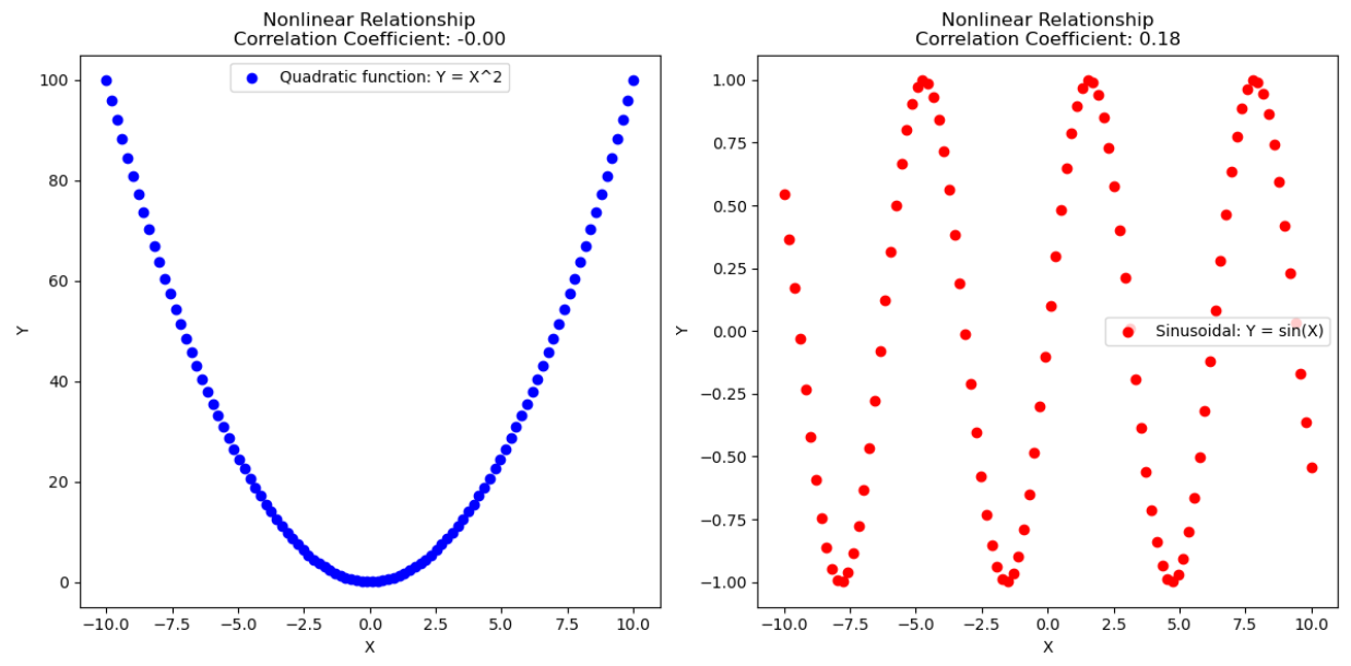Figure: Nonlinear relationship between variables. Source: [4].

10.2 Inferential Statistics

Inferential statistics allow to make predictions or inferences about a population based on a sample of data. Unlike descriptive statistics which simply summarize data, inferential statistics help us draw conclusions and make predictions beyond the immediate data.

Common methods of inferential statistics include:

• Regression analysis, models relationships between variables to make predictions or understand relationships.

• Estimation methods, infer the values of population parameters based on sample data.

• Confidence intervals, provide a range within which a population parameter is expected to lie with a certain level of confidence.

• Hypothesis testing, tests hypotheses about population parameters using statistical tests (e.g., t-tests, chi-square tests, ANOVA (Analayis of Variance)).

10.2.1 Linear Regression

The concept of linear regression has similarities to the Pearson correlation coefficient, as the goal is to examine whether there is a linear relationship between variables. However, regression models are more powerful tools than the measures of correlation.

Given two sets of observations x and y, a linear regression model returns a regression line:

\(\hat{y_i} = b_0 + b_1x_i\)

The values \(b_0\) and \(b_1\) are regression coefficients and represent the intercept of the regression line with the y-axis and the slope of the line, respectively. The regression coefficients are also called the weights of the regression model.

A linear regression model estimates the values of the regression coefficients \(b_0\) and \(b_1\) for a given dataset, as shown in the figure below. The objective is to find the set of regression coefficients so that for all data \(x_i\), the obtained values from the regression equation for the variable \(\hat{y_i}\) are as close as possible to the actual values \(y_i\). The variable x is called independent variable, or it is also called input variable, or observed variable. The variable y is called dependent variable, or predicted variable, or target variable, since the objective is to predict the values of y for given observations x.

One common approach for calculating the regression coefficients is by minimizing the sum of the squared differences between the predicted values \(\hat{y_i}\) and actual values \(y_i\), i.e., \(\sum_{i} (\hat{y_i}-y_i)^2\) for \(𝑖 = 1, 2, …, 𝑛\). This approach is called the method of ordinary least squares. The differences between the predicted values \(\hat{y_i}\) and actual values \(y_i\) are also referred to as residuals.

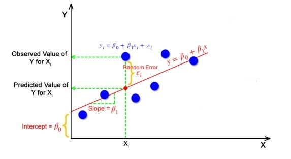Figure: Linear regression. Source: [7].

In scipy we can use the function scipy.stats.linregress to perform linear regression. The result is shown below, and as we can see, the returned values are the slope and intercept of the regression line, rvalue is the correlation coefficient, pvalue is the probability of the linear relationship between the variables, and stderr and intercept_stderr are standard deviations associated with the uncertainties in estimating the slope and intercept of the regression line, respectively.

# SciPy
scipy.stats.linregress(xarr, yarr)

LinregressResult(slope=0.5181818181818181, intercept=5.714285714285714, rvalue=0.861950005631606, pvalue=5.122760847201164e-07, stderr=0.06992387660074979, intercept_stderr=0.4234100995002589)

To access specific values from the result of scipy.stats.linregress(), we can use the dot notation, as in the next cell.

result = scipy.stats.linregress(xarr, yarr)
print(result.slope, result. intercept, result.rvalue)

0.5181818181818181 5.714285714285714 0.861950005631606

Another library for perfroming linear regression is scikit-learn, which we will use extensively later in this course. To quickly demonstrate linear regression, in the next cell we imported the model LinearRegression(), and used the method fit() to apply a linear regression model to the data. For this example we introduced new data variables, where the independent variable is hours and refers to the hours of study for an exam, and the dependent variable is marks representing the obtained score from the exam. We assume that there is a linear relationship between the hours of the study and the exam marks.

hours = np.array([1, 2, 3, 4, 5])
marks = np.array([52, 54, 61, 68, 72])

# scikit-learn
from sklearn.linear_model import LinearRegression

model = LinearRegression()
model.fit(hours.reshape((-1, 1)), marks)

LinearRegression()

In a Jupyter environment, please rerun this cell to show the HTML representation or trust the notebook.
On GitHub, the HTML representation is unable to render, please try loading this page with nbviewer.org.

We can access the slope and intercept regression coefficients of the model through the attributes coef_ and intercept_ of the model.

print(model.coef_, model.intercept_)

[5.4] 45.19999999999999

Now we can use the linear regression model \(\hat{y_i} = b_0 + b_1x_i\) to make predictions for the marks based on given values hours in the dataset.

marks_pred = model.intercept_ + model.coef_ * hours

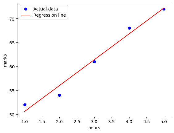
In the following cell, we plotted the actual data with blue markers and the obtained regression line with red color. The intercept with the y-axis is not shown in the plot, but we can notice that for marks=0 the intercept would be around 45 as obtained in the previous cell. I.e., if the student studies 0 hours, the expected score is 45 marks. The slope of the regrestion line is 5.4, meaning that for each additional hour of study, the exam score is expected to increase by about 5.4 marks.

plt.scatter(hours, marks, color='blue', label='Actual data')
plt.plot(hours, marks_pred, color='red', label='Regression line')
plt.xlabel('hours')
plt.ylabel('marks')
plt.legend()
plt.show()

The linear regression model in scikit-learn can also be applied to pandas DataFrames, besides NumPy arrays.

We will learn more about regression models in the subsequent lectures in this course. Here we covered an example of linear regression with one dependent and one independent variable, which is also referred to as simple linear regression, and is an example of a univariate regression. It is possible to consider multiple independent variables (e.g., using multiple input features) to predict another variable, referred to as multiple regression. And the problem of predicting the value of multiple dependent variables is called multivariate regression.

Besides linear regression models which fit a line to a dataset, there are numerous non-linear regression models that fit a non-linear model to a dataset. Later in the course we will study non-linear regression models, such as Random Forest regression model, Support Vector regression model, Neural Networks, and other models.

10.2.1.1 Evaluating the Fit of a Regression Model

Commonly used metrics for evaluating if the regression model is a good fit to a dataset are:

• \(R\)-Squared value (coefficient of determination)

• Mean Squared Error (MSE)

• Root Mean Squared Error (RMSE)

• Mean Absolute Error (MAE)

10.2.1.2 \(R\)-Squared Value (Coefficient of Determination)

\(R\)-Squared value or \(R^2\) is also known as the coefficient of determination. \(R\)-Squared measures how well the independent variable (e.g., hours) explains the variability of the dependent (predicted) variable (marks, in this case). Its value ranges from 0 to 1, where 0 means that the variance in the predicted variable is not explained by the model, and indicates a poor regression fit. Conversely, 1 means that the variance in the predicted variable is well explained by the model, and indicates a good fit where the predicted exam marks are close to the actual values of the exam marks.

The coefficient of determination is calculated as:

\(R^2 = 1 - \frac{\sum_{i=1}^{n} (y_i - \hat{y}_i)^2}{\sum_{i=1}^{n} (y_i - \bar{y})^2}= 1 - \frac{RSS}{TSS}\)

The term in the numerator is called Residual Sum of Squares (RSS), and it is the sum of the squared differences for the residuals, i.e., between each actual value and the corresponding predicted value. It measures the variance that is not explained by the model. The term in the denominator is called Total Sum of Squares (TSS), and it is the sum of the squared differences between each actual value and the mean of the actual values. It measures the total variance in the dependent variable (exam marks). Overall, the R-squared equation measures the proportion of variance in the dependent variable (exam marks) that is predictable from the independent variable (hours) in a regression model.

To calculate \(R\)-Squared, we can import r2_score from scikit-learn, and apply it by using the actual and the predicted values by a model. In this case, the value is 0.97, which means that 97% of the variance in the variable marks is explained by the hours studied. This suggests that the regression model is quite effective in predicting the exam marks based on the hours studied.

# scikit-learn
from sklearn.metrics import r2_score

r2 = r2_score(marks, marks_pred)
print(r2)

0.9745989304812834

For a simple linear regression with one independent variable, \(R\)-Squared is equal to the squared value of the Pearson correlation coefficient, i.e., \(R^2=r^2\). Recall again that the correlation coefficient measures the strength and direction of the linear relationship between two variables, and it ranges from -1 to 1. \(R\)-Squared measures how well a regression model explains the variability in the predicted variable, and it ranges from 0 to 1.

10.2.1.3 Mean Squared Error (MSE) and Root Mean Squared Error (RMSE)

Mean Squared Error (MSE) is calculated as the average of the squared differences between the actual and predicted values.

\(\text{MSE} = \frac{1}{n} \sum_{i=1}^{n} (y_i - \hat{y}_i)^2\)

Root Mean Squared Error (MSE) is the square root of MSE. An advantage of RMSE in comparison to MSE is that it represents the error in the same units as the target variable.

\(\text{RMSE} = \sqrt{\frac{1}{n} \sum_{i=1}^{n} (y_i - \hat{y}_i)^2}\)

MSE can be calculated by importing mean_squared_error from scikit-learn, and RMSE then is calculated as the square root of MSE.

# scikit-learn
from sklearn.metrics import mean_squared_error

mse = mean_squared_error(marks, marks_pred)
print(mse)

1.5199999999999976

rmse = mse ** 0.5
print(rmse)

1.2328828005937944

10.2.1.4 Mean Absolute Error (MAE)

Mean Absolute Error (MAE) is calculated as the average of the absolute differences between the actual and predicted values. It quantifies how far predictions are from the true values.

\(\text{MAE} = \frac{1}{n} \sum_{i=1}^{n} |y_i - \hat{y}_i|\)

MAE can also be imported from scikit-learn.

# scikit-learn
from sklearn.metrics import mean_absolute_error

mae = mean_absolute_error(marks, marks_pred)
print(mae)

1.0399999999999991

Smaller values of MSE, RMSE, and MAE are indicators of a better regression fit, and greater values of \(R\)-squared represent a better regression fit.

10.2.2 Standard Error of the Mean

The standard error estimates the variability of a sample statistic from the true population parameter. A commonly used standard error measure is for the sample mean.

The standard error of the mean (SEM) is an inferential statistic that measures the variability of the sample mean as an estimate of the true population mean. It is often used in estimation methods, confidence intervals, and hypothesis testing.

The SEM is the standard deviation of the sampling distribution of the sample mean. It quantifies how much the sample mean is expected to fluctuate from the true population mean if we repeatedly draw new samples from the population.

To calculate SEM, we use the following formula:

\(\text{SEM} = \frac{\sigma}{\sqrt{n}}\)

In the formula, \(\sigma\) is the population standard deviation and \(𝑛\) is the sample size. If the population standard deviation is unknown, the sample standard deviation \(s\) is used.

The SEM provides insight into the reliability of the sample mean as an estimate of the population mean. A smaller SEM indicates a more precise estimate, which is valuable for making statistical inferences.

In Python, we can calculate the standard error of the mean via the sem() function in scipy.stats. Large value of the standard error of the mean indicates more spread out values around the mean of the data.

data = [3, 4, 4, 5, 7, 8, 12, 14, 14, 15, 17, 19, 22, 24, 24, 24, 25, 28, 28, 29]

# SciPy
scipy.stats.sem(data)

2.0014468450808804

np.mean(data)

16.3

Since the standard error of the mean depends on the sample size \(n\), as the sample size increases, the standard error of the mean tends to decrease.

10.2.3 Confidence Intervals

A confidence interval is a range of values derived from sample data that provides an estimate of a population parameter. The confidence level represents the degree of certainty that the interval contains the true population pararameter. For example, a 90% confidence level indicates that if the same sampling process is repeated multiple times, approximately 90 out of 100 times the confidence intervals would contain the true population mean.

The confidence interval (CI) for the population mean is calculated with the following formula.

\(\text{CI} = \bar{x} \pm Z \cdot \frac{\sigma}{\sqrt{n}}\)

In the formula, \(\bar{x}\) is the sample mean, \(\sigma\) is the population standard deviation, \(n\) is the sample size, and \(Z\) is the Z-score corresponding to the desired confidence level. Notice that the CI depends on the standard error of the mean (\(\text{SEM} = {\sigma}/{\sqrt{n}}\)), and it can also be written as \(\text{CI} = \bar{x} \pm Z \cdot \text{SEM}\).

The Z-score is a statistical measure that quantifies how many standard deviations a data point is from the mean of a distribution. It is a method for standardizing scores on a normal distribution. For a given value \(x\) in a dataset with mean \(\bar{x}\) and standard deviation \(\sigma\), the Z-score is calculated as:

\(Z = \frac{x - \bar{x}}{\sigma}\)

Example of Z-scores for Confidence Intervals:

• 95% Confidence Interval: the Z-score corresponds to the critical value that leaves 2.5% in each tail of the normal distribution. The Z-score for a 95% confidence interval is approximately ±1.96. The figure below depicts the 95% confidence interval for the sample mean.

• 99% Confidence Interval: the Z-score corresponds to the critical value that leaves 0.5% in each tail of the normal distribution. The Z-score for a 99% confidence interval is approximately ±2.58.

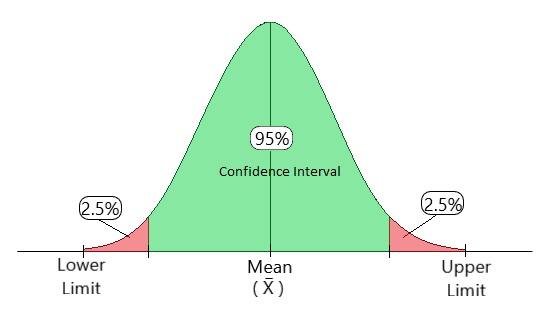Figure: 95% confidence interval..

All statistical software packages provide Z-scores for a desired confidence level. Additionally, Z-scores can be read from normal distribution tables, also called Z-tables. For example, to find the Z-score for a 95% confidence level, we need to locate the value in the table that leaves 2.5% in each tail, which corresponds to ±1.96.

In the next example, we first draw 100 samples from a random uniform distribution having integer values between 5 and 10. Next, we calculate the sample mean and the standard error of the mean. Afterward, we use the norm.interval() function from scipy.stats to calculate the confidence interval. Arguments in the function are the confidence interval (set to 90%), the sample mean, and the standard error of the mean.

# SciPy
sample_data = np.random.randint(5, 10, 100)

# sample mean
sample_mean = np.mean(sample_data)
# standard error of the mean
sample_sem = scipy.stats.sem(sample_data)

# 90% confidence interval for population mean
confidence_interval = scipy.stats.norm.interval(confidence=0.90, loc=sample_mean, scale=sample_sem)

In the next cell, the sample mean is 6.77, and the 90% confidence interval is from 6.55 to 6.99.

print(sample_mean)
print(confidence_interval)

7.1
(6.873936491913292, 7.326063508086707)

In the next cell we set the confidence level to 99%, that is, we want to be 99% sure the interval contains the true population mean. The resulting CI is between 6.39 and 7.15, and it is a wider interval because we are trying to capture the true mean with greater certainty, accounting for more possible variation in the data.

# 99% confidence interval for population mean
confidence_interval = scipy.stats.norm.interval(confidence=0.99, loc=sample_mean, scale=sample_sem)

print(sample_mean)
print(confidence_interval)

7.1
(6.74598612359689, 7.454013876403109)

If the population standard deviation \(\sigma\) is unknown, we can use the sample standard deviation \(s\) to calculate the CI using the following formula:

\(\text{CI} = \bar{x} \pm t \cdot \frac{s}{\sqrt{n}}\)

In this case, a \(t\)-score from the \(t\)-distribution is used that corresponds to the desired confidence level.

Additionally, if the sample size is small and it is below 30 data points, the above formula based on \(t\)-score is used for calculating the CI.

Let’s create a smaller dataset containing 16 data points first. We can calculate the confidence interval by using the t.interval() function from scipy.stats. The rest of the code is similar to the above cell, with the only difference that there is one additional parameter corresponding to the degree of freedom of the data.

sample_data = [1, 1, 1, 2, 2, 3, 3, 3, 4, 4, 5, 5, 6, 7, 8, 10]

# sample mean
sample_mean = np.mean(sample_data)
# standard error of the mean
sample_sem = scipy.stats.sem(sample_data)
# degrees of freedom
sample_df = len(sample_data)-1

# create 90% confidence interval
confidence_interval = scipy.stats.t.interval(confidence=0.90, loc=sample_mean, scale=sample_sem, df=sample_df)

print(sample_mean)
print(confidence_interval)

4.0625
(2.903311331486366, 5.221688668513634)

10.2.4 Hypothesis Testing

Hypothesis testing is a fundamental statistical technique for making inferences about populations based on sample data.

Hypothesis testing involves two main hypotheses:

• Null Hypothesis (\(H_0\)): it is the default hypothesis that there is no change, difference, or effect in the value(s) of the studied statistic(s), and any observed result is due to random chance. It serves as the baseline against which the alternative hypothesis is tested. For example, in a drug efficacy test, the null hypothesis can be “The drug has no effect on patients.”

• Alternative Hypothesis (\(H_1\), or \(H_a\)): it is the opposite of the null hypothesis, and suggests that there is a change, difference, or effect in the value(s) of the studied statistic(s), and the observed result is not due to random chance. For the example with the drug test, the alternative hypothesis can be “The drug has a significant effect on patients.”

Therefore, the test evaluates two opposing hypotheses. Based on the results of the test, either the null hypothesis \(H_0\) is rejected (suggesting that the alternate hypothesis \(H_a\) is supported, and there is evidence of a difference), or the null hypothesis \(H_0\) is not rejected (suggesting that the alternative hypothesis \(H_a\) is not supported, and there is no evidence of a difference).

To test the hypotheses, we need to select a level of significance of the test, typically denoted by \(\alpha\). Common choices for the level of significance are 1%, 5%, or 10%. In most practical tests, a level of significance equal to 5% (\(\alpha=0.05\)) is selected. The level of significance represents the probability of making a Type I error, which occurs when the null hypothesis is rejected even though it is true.

The value of \((1 − 𝛼)\) is called confidence level, and it represents the degree of certainty we have in our test results. For example, if \(𝛼=0.05\) (5%), the corresponding confidence level is \(1 − 0.05 = 0.95\), meaning that we are 95% confident that the observed results are not due to random chance.

The output of a hypothesis test typically includes the value of the test statistics and a significance probability, commonly referred to as the \(p\)-value. If the \(p\)-value is less than or equal to the level of significance \(\alpha\) (e.g., 0.05), the null hypothesis is rejected. Conversely, if the \(p\)-value is greater than the level of significance \(\alpha\), this indicates that the observed data is consistent with the null hypothesis, and there is insufficient evidence to reject the null hypothesis.

For example, if we select \(\alpha\) = 0.05 and the obtained \(p\)-value from the test is 0.1, we can conclude that we fail to reject the null hypothesis at the 95% confidence level. Or, we can say that there is no statistically significant difference between the population parameter and the sample statistic at the 95% confidence level.

Several types of hypothesis tests are used depending on the given data and research question. The following are common hypothesis tests.

One-Sample t-Test

One-sample \(t\)-test is used to determine whether the mean of a population is significantly different from a specific value.

For instance, a pharmaceutical company claims that a new drug lowers blood pressure on average by 10 mmHg. The drug can be administered to 20 patients and measure their blood pressure. A one-sample \(t\)-test can be used to determine if the measured pressure of the patients is statistically different from the expected reduction of 10 mmHg.

The \(t\)-statistic is calculated as:

\(t = \frac{\bar{x} - \mu_0}{\frac{s}{\sqrt{n}}}\)

where \(\bar{x}\) is the sample mean, \(\mu_0\) is the population mean under the null hypothesis, \(s\) is the sample standard deviation, and \(n\) is the sample size.

# SciPy
# Sample data
data = np.array([2.3, 2.8, 2.5, 2.7, 3.1, 2.6])

# Null hypothesis: mean = 2.5
t_statistic, p_value = scipy.stats.ttest_1samp(data, 2.5)

print(t_statistic, p_value)

if p_value < 0.05:
    print("Reject the null hypothesis")
else:
    print("Fail to reject the null hypothesis")

1.4940357616679902 0.19539449179127277
Fail to reject the null hypothesis

np.mean(data)

2.6666666666666665

Since the \(p\)-value is greater than 0.05, we fail to reject the null hypothesis that the mean of data is 2.5, meaning there is no significant difference from 2.5.

Two-Sample t-Test

This test is used to compare the means of two independent samples.

For example, a medical study aims to compare the blood pressure of two groups of patients, consisting of people under 40 and over 60. A two-sample \(t\)-test can be used to determine if there is a statistically significant difference in the average blood pressure between the two groups of patients.

The \(t\)-statistic is calculated as:

\(t = \frac{\bar{x}_1 - \bar{x}_2}{\sqrt{\frac{s_1^2}{n_1} + \frac{s_2^2}{n_2}}}\)

where \(\bar{x}_1\) and \(\bar{x}_1\) are the sample means, \(s_1\) and \(s_2\) are the standard deviations, and \(n_1\) and \(n_2\) are the sample sizes.

# SciPy
# Sample data
data1 = np.array([2.3, 2.8, 2.5, 2.7, 3.1, 2.6])
data2 = np.array([3.2, 3.5, 3.6, 3.7, 3.8, 3.9])

# Null hypothesis: means of data1 and data2 are equal
t_statistic, p_value = scipy.stats.ttest_ind(data1, data2)

print(t_statistic, p_value)

if p_value < 0.05:
    print("Reject the null hypothesis")
else:
    print("Fail to reject the null hypothesis")

-6.302287394737564 8.882097195524333e-05
Reject the null hypothesis

Since the \(p\)-value is less than 0.05, we reject the null hypothesis that the means of data1 and data2 are equal, and we conclude that the two sample means are significantly different.

Paired t-Test

Paired \(t\)-test is used to compare the means of two related groups. For instance, when we have two measurements taken on the same sample or matched pairs before and after an intervention or change.

For example, the same group of patients undergoes a new treatment for 8 weeks, and their blood pressure levels are measured before and after the treatment. A paired \(t\)-test can be used to determine if there is a statistically significant difference in the measured blood pressure levels before and after the treatment.

The \(t\)-statistic is calculated as:

\(t = \frac{\bar{d}}{\frac{s_d}{\sqrt{n}}}\)

where \(\bar{d}\) is the mean difference between paired observations, \(s_d\) is the standard deviation of the differences, and \(n\) is the number of pairs.

# SciPy
# Sample data
before = np.array([2.3, 2.8, 2.5, 2.7, 3.1, 2.6])
after = np.array([2.4, 2.9, 2.7, 2.8, 3.2, 2.7])

# Null hypothesis: means of before and after are equal
t_statistic, p_value = scipy.stats.ttest_rel(before, after)

print(t_statistic, p_value)

if p_value < 0.05:
    print("Reject the null hypothesis")
else:
    print("Fail to reject the null hypothesis")

-6.9999999999999885 0.0009167475143984109
Reject the null hypothesis

The p-value is less than 0.05, therefore we reject the null hypothesis that the means are equal, and we conclude that the difference between the means before and after the intervention is statistically significant.

Chi-Square Test

Chi-square test is used for categorical data to assess how likely it is that observed frequencies in one or more categories match expected frequencies.

For example, a political researcher has collected tabular data with voting preferences for two candidates. The researcher can use a chi-square test to examine if the gender of the voters (male vs female) is associated with their voting preference for the two candidates.

The test statistic is calculated as:

\(\chi^2 = \sum \frac{(O_i - E_i)^2}{E_i}\)

where \(O_i\) are the observed frequencies, and \(E_i\) are the expected frequencies.

# SciPy
# Sample data: Observed frequencies
observed = np.array([30, 10, 20, 40])

# Expected frequencies
expected = np.array([25, 25, 25, 25])

# Null hypothesis: observed and expected frequencies are equal
chi2_statistic, p_value = scipy.stats.chisquare(observed, expected)

print(chi2_statistic, p_value)

if p_value < 0.05:
    print("Reject the null hypothesis")
else:
    print("Fail to reject the null hypothesis")

20.0 0.00016974243555282632
Reject the null hypothesis

The \(p\)-value is less than 0.05, therefore we reject the null hypothesis, and conclude that the observed frequencies differ significantly from the expected ones.

References

1. Python Statistics Fundamentals: How to Describe Your Data, by Mirko Stojiljković, available at: https://realpython.com/python-statistics/.

2. Learning Statistics with Python, by Ethan Weed, available at: https://ethanweed.github.io/pythonbook/landingpage.html#.

3. Correlation Coefficients: Appropriate Use and Interpretation, by Patrick Schober, Christa Boer, and Lothar A Schwarte, available at: https://pubmed.ncbi.nlm.nih.gov/29481436/

4. Linear and Nonlinear Correlations, available at: https://rovusa.com/quantitative-statistical-methods-and-data-science/linear-and-nonlinear-correlations/.

5. Mastering Statistical Analysis in Python with Real-World Datasets, by Ratan Kumar Sajja, available at: https://python.plainenglish.io/mastering-statistical-analysis-in-python-with-real-world-datasets-d5b60e541189.

6. Applying Descriptive and Inferential Statistics in Python, by Cornellius Yudha Wijaya, available at: https://www.kdnuggets.com/applying-descriptive-and-inferential-statistics-in-python.

7. Linear Regression: A Comprehensive Guide, Analytics Vidhya, available at: https://www.analyticsvidhya.com/blog/2021/10/everything-you-need-to-know-about-linear-regression/.

BACK TO TOP